Mathematical Models In Population Biology And Epidemiology Solutions Manual Pdf

Article Menu

/ajax/scifeed/subscribe

Open Access Editor's Choice Article

A Mathematical Model of Epidemics—A Tutorial for Students

Department of Physics, Tokyo Metropolitan University, Hachioji, Tokyo 192-0397, Japan

^*

Author to whom correspondence should be addressed.

Received: 10 June 2020 / Revised: 10 July 2020 / Accepted: 14 July 2020 / Published: 17 July 2020

Abstract

This is a tutorial for the mathematical model of the spread of epidemic diseases. Beginning with the basic mathematics, we introduce the susceptible-infected-recovered (SIR) model. Subsequently, we present the numerical and exact analytical solutions of the SIR model. The analytical solution is emphasized. Additionally, we treat the generalization of the SIR model including births and natural deaths.

1. Introduction

The coronavirus disease 2019 (COVID-19) is an infectious disease that emerged in Wuhan, China in December 2019 and has rapidly spread in China and worldwide. On 30 January 2020, the World Health Organization (WHO) declared the outbreak as a public health emergency of international concern. Furthermore, the WHO announced the COVID-19 outbreak as a "pandemic" on 11 March 2020 [1,2]. The prevention of infection is the responsibility of every human being.

A few mathematical models have been developed to describe the dynamics of the evolution of COVID-19 [3,4,5,6,7]. Among them, the susceptible-infected-recovered (SIR) model is treated as a basic mathematical model for the spread of epidemic diseases. This model was proposed in 1927 by Kermack and McKendrick [8,9], and has been used as a basic model for epidemics [10,11,12,13,14].

The SIR model is not difficult from the viewpoint of mathematics, and can be understood even by high-school students. We present a numerical solution and an exact analytical solution [15] of the SIR model herein. The analytical solution is emphasized because it is not well known. We provide a more straightforward derivation of the analytical solution compared with that in the original paper; it will serve as a good opportunity for students to learn differentiation and integration. Furthermore, we treat the generalization of the SIR model with vital dynamics including birth and natural death processes. We demonstrate that the complex SIR model can be reduced to an Abel-type differential equation.

2. Exponential Growth

The spread of an epidemic disease depends on both the amount of contact between individuals and the possibility of an infected person transmitting the disease to another person. If each infected person is in contact with two other people before they recover, the disease will soon begin to spread rapidly. Assuming that recovery requires one day, the number of sick people will double each day. This situation is illustrated schematically in Figure 1. A numerical series for which the ratio of each two consecutive terms is a constant r (in this case,

$r=2$

) is called a geometric series. The n-th term is expressed as follows:

$$A\left(n\right)=A\left(0\right)r^n,$$

(1)

where the initial value is set to be

$A\left(0\right)$

. If r is greater than 1, then the series increases and approaches positive infinity rapidly (we assume

$A\left(0\right)>0$

); if r is smaller than 1, the series decreases and approaches zero. At the border of

$r=1$

, the series remains constant. As an example, when one borrows money, the interest is typically a compound interest, i.e., a geometric series. When the annual interest is 30%, the return in five years will increase rapidly as follows:

$$\frac{A\left(5\right)}{A\left(0\right)}=1.3^5\simeq 3.7.$$

(2)

Extending n to a real number, we introduce the exponential function

The differentiation of the exponential function can be calculated as follows:

$$\frac{dx}{dt}=\underset{h\to 0}{lim}\frac{r^{t+h}-r^t}{h}=r^t\underset{h\to 0}{lim}\frac{r^h-1}{h}.$$

(4)

The special constant r that satisfies the limiting equation

$$\underset{h\to 0}{lim}\frac{r^h-1}{h}=1$$

(5)

is called Napier's constant e. With this definition of e, the differentiation of the exponential function becomes

Hereafter, we treat the form of the exponential function as

The exponential function grows for

$a>0$

, and decays for

$a<0$

. When

$a=0$

, the function becomes constant. We have assumed that

$C>0$

.

The inverse function of x,

$t=t\left(x\right)$

, is a logarithmic function written as

where r is the base. The logarithmic function with the base e is called a natural logarithmic function and is denoted as follows:

The exponential function always explodes for

$a>0$

. To verify whether it grows rapidly or slowly, we may consider the doubling time. From the condition

$$\frac{x\left(t_2\right)}{x\left(t_1\right)}=\frac{e^{a{t}_2}}{e^{a{t}_1}}=e^{a(t_2-t_1)}=2,$$

(10)

we obtain that the doubling time is a time difference that satisfies

$$a(t_2-t_1)=ln2.$$

(11)

It is instructive to use graph plots to observe the growth behavior. Both the linear and semi-log plots are shown in Figure 2. A semi-log plot has one axis (t) on a linear scale, and the other on a logarithmic scale. When the function grows exponentially, a linear increase is observed in a semi-log plot.

Next, we explain the differential equation. Let us consider the case in which the increase in a variable

$x\left(t\right)$

is proportional to

$x\left(t\right)$

, i.e.,

$$\Delta x\left(t\right)=x(t+\Delta t)-x\left(t\right)=ax\left(t\right)\Delta t.$$

(12)

The difference in the left-hand side becomes larger when the time difference

$\Delta t$

becomes longer; hence,

$\Delta t$

is multiplied to the right-hand side. If we divide both sides by

$\Delta t$

and take the limit of

$\Delta t\to 0$

, the following differentiation definition is obtained:

$$\underset{\Delta t\to 0}{lim}\frac{x(t+\Delta t)-x\left(t\right)}{\Delta t}=\frac{dx\left(t\right)}{dt}=ax\left(t\right).$$

(13)

It becomes a

$dx\left(t\right)/dt$

equation, which is known as a differential equation. Because Equation (7) satisfies the differential equation, it is regarded as a general solution to the differential equation shown in Equation (13). Here, C is an arbitrary constant and is known as an integral constant. Next, we discuss the mathematical model of the spread of epidemic diseases.

3. Mathematical Model of Epidemics

If exponential growth continues, the number of the infected individuals increases. We may consider that the infected individuals recover and develop immunity. Subsequently, the number of recovered individuals increases, but we hope that the spread of the disease will subside. We may consider a closed society of N individuals and classify individuals into three types: susceptible (S), infected (I), and recovered (R). The SIR model [8,9] is a mathematical model for the spread of epidemic diseases that describes the changes in the numbers of the three types of individuals.

We denote the number of susceptible (S) individuals by

$x\left(t\right)$

, the number of infected (I) individuals by

$y\left(t\right)$

, and the number of recovered or removed (R) individuals by

$z\left(t\right)$

. The time t is measured in days, t (day). We may consider that each person is in contact with m persons per day on average. Because the proportion of infected individuals is

$y\left(t\right)/N$

, the number of contacts between the infected and susceptible persons becomes

$m\left(y\right(t)/N)x\left(t\right)$

per day. If we set the probability of infection for each contact as p, the number of the newly infected individuals within

$\Delta t$

days becomes

$$m\frac{y\left(t\right)}{N}x\left(t\right)p\Delta t$$

(14)

in total. If we set

$\beta =mp$

, the number of non-infected individuals (S) from the t-th day through the (

$t+\Delta t$

)-th day changes as

$$x(t+\Delta t)-x\left(t\right)=-\frac{\beta }{N}x\left(t\right)y\left(t\right)\Delta t.$$

(15)

For the limit of

$\Delta t\to 0$

, the derivative can be obtained as follows:

$$\frac{dx\left(x\right)}{dt}=-\frac{\beta }{N}x\left(t\right)y\left(t\right),$$

(16)

which is the same procedure as that derived for Equation (13).

Meanwhile, the infected individuals recover at a removal rate of

$\gamma$

per day. Subsequently, the increase in the number of the recovered persons becomes

$$\frac{dz\left(t\right)}{dt}=\gamma y\left(t\right).$$

(17)

The inverse of

$\gamma$

is the expected duration of infection. Here, the number of the recovered persons includes the number of the deceased persons because it refers to the number of individuals who cannot possibly infect others.

Because the total number of individuals is set to be constant such that

$$x\left(t\right)+y\left(t\right)+z\left(t\right)=N,$$

(18)

we express

$y\left(t\right)$

as follows:

$$y\left(t\right)=N-x\left(t\right)-z\left(t\right).$$

(19)

The change in the number of the infected individuals can be written as

$$\frac{dy\left(t\right)}{dt}=-\frac{dx\left(t\right)}{dt}-\frac{dz\left(t\right)}{dt}=\frac{\beta }{N}x\left(t\right)y\left(t\right)-\gamma y\left(t\right).$$

(20)

Gathering the equations, we have

$$\begin{array}{cc}\hfill \frac{dx\left(t\right)}{dt}& =-\frac{\beta }{N}x\left(t\right)y\left(t\right),\hfill \end{array}$$

(21)

$$\begin{array}{cc}\hfill \frac{dy\left(t\right)}{dt}& =\frac{\beta }{N}x\left(t\right)y\left(t\right)-\gamma y\left(t\right)=\left(\frac{\beta }{N}x\left(t\right)-\gamma \right)y\left(t\right),\hfill \end{array}$$

(22)

$$\begin{array}{cc}\hfill \frac{dz\left(t\right)}{dt}& =\gamma y\left(t\right).\hfill \end{array}$$

(23)

These are simultaneous equations, where

$\beta$

is the rate of infection and

$\gamma$

the rate of recovery (the rate of quarantine).

If we introduce the transformations of variables, such as

$\tilde{x}=x/N,\tilde{y}=y/N,\tilde{z}=z/N$

, and

$\tilde{t}=\beta t$

, then Equations (21)–(23) can be rewritten as

$$\begin{array}{cc}\hfill \frac{d\tilde{x}\left(t\right)}{d\tilde{t}}& =-\tilde{x}\left(t\right)\tilde{y}\left(t\right),\hfill \end{array}$$

(24)

$$\begin{array}{cc}\hfill \frac{d\tilde{y}\left(t\right)}{d\tilde{t}}& =\left(\tilde{x}\left(t\right)-\frac{1}{R_0}\right)\tilde{y}\left(t\right),\hfill \end{array}$$

(25)

$$\begin{array}{cc}\hfill \frac{d\tilde{z}\left(t\right)}{d\tilde{t}}& =\frac{1}{R_0}\tilde{y}\left(t\right).\hfill \end{array}$$

(26)

The equations are in non-dimensional forms. The use of

$\tilde{x},\tilde{y}$

, and

$\tilde{z}$

implies that we only need to consider the fraction of the number of individuals. A single parameter representing the ratio of

$\beta$

and

$\gamma$

appears as follows:

The number

$R_0$

is known as the basic reproduction number [16,17,18], and the number of infected individuals increases when

$R_0>1$

(precisely, in the limit of

$\tilde{x}\left(0\right)\to 1$

), whereas it decreases when

$R_0<1$

.

4. Numerical Solution of SIR Model

The SIR equations (Equations (21)–(23)) were derived; subsequently, the differential equations can be solved numerically. The simplest method to solve the differential equation is as follows: It is noteworthy that

$$x(t+\Delta t)-x\left(t\right)\simeq \frac{dx\left(t\right)}{dt}\Delta t.$$

(28)

Therefore, we may calculate

$$x(t+\Delta t)\simeq x\left(t\right)+\frac{dx\left(t\right)}{dt}\Delta t$$

(29)

with a time step size of

$\Delta t$

. This first-order numerical procedure is known as the Euler method. However, it has a convergence problem; therefore, the errors will be larger. Although many methods have been proposed to reduce errors, we employ the second-order Runge–Kutta method.

The python program is given in Appendix A. As initial conditions, we use

with

$N=10,000,N_1=9900,N_2=10$

, and

$N_3=0$

. The calculated results using parameters

$\beta =0.5$

and

$\gamma =0.2$

are shown in Figure 3a. As shown, the number of infected individuals (I) increases with time, reaches a peak, and gradually decreases. Meanwhile, the number of the recovered individuals (R) increases gradually.

Thus far, we have discussed the number of the infected individuals,

$y\left(t\right)$

. The number of newly infected individuals is reported daily. How can we express the number of the newly infected individuals in the framework of the SIR model? The newly infected individuals are added to

$y\left(t\right)$

, but the recovered individuals

$z\left(t\right)$

are subtracted from

$y\left(t\right)$

as well. Therefore, the number of the newly infected individuals,

$y_{\mathrm{new}}\left(t\right)$

, is expressed as

$$y_{\mathrm{new}}\left(t\right)=(y\left(t\right)+z\left(t\right))-(y(t-\Delta t)+z(t-\Delta t))$$

(33)

with

$\Delta t=1$

. Because

$x\left(t\right)+y\left(t\right)+z\left(t\right)=N$

, we can express

$$y_{\mathrm{new}}\left(t\right)=-(x\left(t\right)-x(t-\Delta t)).$$

(34)

Based on Equation (21), we obtain

$$y_{\mathrm{new}}\left(t\right)\simeq -\frac{dx\left(t\right)}{dt}\Delta t=\frac{\beta }{N}x\left(t\right)y\left(t\right)\Delta t.$$

(35)

Because

$y_{\mathrm{new}}\left(t\right)$

is proportional to

$y\left(t\right)$

, the behavior of the temporal variation of

$y_{\mathrm{new}}\left(t\right)$

is similar to that of

$y\left(t\right)$

. In Figure 3a,

$y_{\mathrm{new}}\left(t\right)$

is plotted as a dotted red curve.

In Figure 3b, the temporal variations of the numbers of individuals for the three types (S, I, R) are compared for

$\beta$

= 0.5, 0.45, 0.4, 0.35, and 0.3. Here,

$\gamma$

is fixed as 0.2. The delay of the epidemic and the reduction in the peak height (number of the infected individuals) were shown as

$\beta$

decreases. This trend is typically associated with the effect of social distancing.

The basic reproduction number

$R_0$

is frequently used as the "R naught" or "R zero". Sometimes, it is treated as a time-varying variable and used as a measure for easing lockdowns. In the SIR model,

$R_0$

is a constant and defined as shown in Equation (27). If we formally define a time-varying number as

$$R_0\left(t\right)=\left(\frac{\beta }{\gamma }\right)\left(\frac{x\left(t\right)}{N}\right),$$

(36)

in the framework of the SIR model, it judges whether

$y\left(t\right)$

increases (

$R_0\left(t\right)>1$

) or decreases (

$R_0\left(t\right)<1$

) in Equation (22). In Figure 3a, this time-varying

$R_0\left(t\right)$

is also plotted as a dotted black curve. The initial value

$R_0$

was set to be 2.5; as shown,

$R_0\left(t\right)$

gradually decreases, becomes 1 at the point where

$y\left(t\right)$

reaches a peak, and further decreases below 1. The terminology "effective reproduction number" is sometimes used, but it has several meanings.

Finally, we remark on the cumulative number of the infected individuals, which is reported daily. In this model, the cumulative number is expressed as

$y\left(t\right)+z\left(t\right)$

because it includes the number of the recovered individuals. In the initial stage of the outbreak of an epidemic, this number increases exponentially, and it is appropriate to use the semi-log plot as shown in Figure 2b. The initial increase in the cumulative number of the infected individuals,

$y\left(t\right)+z\left(t\right)$

, is plotted in a semi-log plot for several

$\beta$

in Figure 4, where

$\gamma$

is fixed. As shown, the initial increase is linear, and the slope decreases as

$\beta$

decreases.

5. Analytical Solution of SIR Model

We have demonstrated the numerical solution of the SIR model. Although the SIR model was proposed in 1927 [8,9], the analytical solution of the differential equations was only presented in 2014 [15]. In the analytical solution, only exponential and logarithmic functions are involved. Therefore, high-school students will be able to understand the analytical solution of the SIR model.

Next, we present the main stream of the derivation of the analytical solution. Some detailed calculations are given as questions, and the solutions can be found in Appendix B. Equations (21)–(23) are simultaneous differential equations; we can rewrite them as the differential equation of a single function. The procedure is the same as that used to solve a linear simultaneous equation.

We employ a more direct method of deriving the analytical solution compared with that in the original paper [15]. First, we rewrite Equation (21) as

where

$\widehat{\beta }=\beta /N$

. If we differentiate both sides, we obtain

$$y^{\prime }=-\frac{1}{\widehat{\beta }}\left(-\frac{x^{\prime 2}}{x^2}+\frac{x^{″}}{x}\right).$$

(38)

Inserting Equation (37) into Equation (21) yields

$$y^{\prime }=-(\widehat{\beta }x-\gamma )\frac{1}{\widehat{\beta }}\left(\frac{x^{\prime }}{x}\right).$$

(39)

Comparing Equation (38) and Equation (39), we have

$$x\frac{d^{2}x}{d{t}^2}-{\left(\frac{dx}{dt}\right)}^2+(\gamma -\widehat{\beta }x)x\frac{dx}{dt}=0.$$

(40)

Therefore, we have obtained a single differential equation of

$x\left(t\right)$

.

Next we introduce the following function:

Therefore, we have the following equation for

$\varphi$

:

$$\frac{d\varphi }{dx}+\frac{\varphi }{x}=(\gamma -\widehat{\beta }x){\varphi }^2.$$

(42)

An ordinary differential equation of this form is known as the Bernoulli differential equation. The general solution is obtained as follows:

$$\varphi =\frac{1}{x(C_1-\gamma lnx+\widehat{\beta }x)},$$

(43)

where

$C_1$

is an integral constant.

Problem1.

Show that the general solution of the Bernoulli differential Equation (42) is given by Equation (43).

From the relation of the inverse function of Equation (41), we have

Using Equation (21), we obtain

$$y=-\frac{1}{\widehat{\beta }}(C_1-\gamma lnx+\widehat{\beta }x).$$

(45)

Moreover, from Equations (21) and (23), we have

$$\frac{dz}{dt}=-\frac{\gamma }{\widehat{\beta }}\left(\frac{x^{\prime }}{x}\right).$$

(46)

Subsequently, the relation between

$x\left(t\right)$

and

$z\left(t\right)$

becomes

$$z\left(t\right)=-\frac{\gamma }{\widehat{\beta }}ln(x\left(t\right)/C_2),$$

(47)

where

$C_2$

is an integral constant. If

$x\left(0\right)=N_1$

and

$z\left(0\right)=0$

for

$t=0$

, then

$C_2$

becomes

$N_1$

. Therefore, we have

$$z=-\frac{\gamma }{\widehat{\beta }}ln(x/N_1).$$

(48)

From the relation

$x\left(0\right)+y\left(0\right)+z\left(0\right)=N$

, we obtain the integral constant

$C_1$

as

$$C_1=-\widehat{\beta }N+\gamma ln{N}_1.$$

(49)

If we substitute

$C_1$

into Equation (43), we have

$$\frac{dt}{dx}=\frac{1}{x(-\widehat{\beta }N-\gamma ln(x/N_1)+\widehat{\beta }x)}.$$

(50)

By integrating this equation, t is obtained as a function of x as follows:

$$t={\int }_{x\left(0\right)}^{x\left(t\right)}\frac{d\xi }{\xi (-\widehat{\beta }N-\gamma ln(\xi /N_1)+\widehat{\beta }\xi )}.$$

(51)

Problem2.

Confirm that Equation (51) satisfies differential Equations (21)–(23).

For the convenience of calculation, we change a variable such that

$\xi /N_1\to \xi$

. Subsequently, we rewrite it as

$$t={\int }_1^{x\left(t\right)/N_1}\frac{d\xi }{\xi (-\beta -\gamma ln\xi +\beta (N_1/N)\xi )}.$$

(52)

It is noteworthy that

$\beta$

appears here instead of

$\widehat{\beta }$

.

Because we have obtained the form of the integral of one variable, we then calculate

$t\left(x\right)$

. We can perform a numerical integration by summing up an integrand with a sufficiently small step size, as follows:

$${\int }_a^{b}f\left(\xi \right)d\xi \simeq \sum _{i=0}^{n-1}f(a+ih)h,h=(b-a)/n.$$

(53)

It is noteworthy that the direction of the integral is negative because

$x\left(t\right)/N_1<1$

in Equation (52), and the integrand has a negative value. If

$t\left(x\right)$

is obtained, then y and z can be calculated using Equations (45) and (48), respectively. The calculated results of

$x\left(t\right),y\left(t\right)$

, and

$z\left(t\right)$

are shown in Figure 5, where the same conditions are used as in Figure 3a. As expected, the analytical solution and the numerical solution obtained using the Runge–Kutta method are the same.

Next, we analyze the property of the differential equation. We can investigate the behavior of

$t\to \infty$

. The variable

$\xi$

in the limit of

$t\to \infty$

,

$x(\infty )/N_1$

, is obtained when the denominator of the integrand of Equation (52) becomes zero. If we write the solution to the equation

$$\beta +\gamma ln\xi -\beta (N_1/N)\xi =0$$

(54)

as

${\xi }^{\ast }$

, we have

$x(\infty )=N_1{\xi }^{\ast }$

,

$y(\infty )=0$

, and

$z(\infty )=N-N_1{\xi }^{\ast }$

. To solve an equation such as Equation (54) numerically, an iterative method such as Newton's method is used. However, for the case of a single variable, it is sufficient to plot the left-hand side of Equation (54) and find an intersection with a zero. Figure 3b shows a comparison of the behaviors of the temporal evolutions of

$x\left(t\right)$

,

$y\left(t\right)$

, and

$z\left(t\right)$

for

$\beta$

= 0.5, 0.45, 0.4, 0.35, and 0.3, with

$\gamma =0.2$

(

$N=10,000,N_1=9900$

). Figure 6 shows the solutions of Equation (54) under the same conditions. The solutions reproduce the limit values of

$x\left(t\right)$

for

$t\to \infty$

in Figure 3b. Using

$R_0$

defined in Equation (27), we can rewrite Equation (54) as

in the limit of

$N_1/N\to 1$

. This relation is known as the solution of the final size equation [19].

The final number of the infected individuals, (

$z(\infty )=N-x(\infty )$

), is a variable of interest. The

$\beta$

dependence of this number is tabulated in Table 1. As shown, the final number of the infected individuals decreases with the infection rate

$\beta$

. Furthermore, the table presents the peak values of the infected individuals.

6. Analytical Approach of SIR Model with Vital Dynamics

The standard SIR model has been extended to include some other factors. One example is a model that considers birth and natural death processes [20,21]. The nonlinear equations are as follows:

$$\begin{array}{cc}\hfill \frac{dx\left(t\right)}{dt}& =-\widehat{\beta }x\left(t\right)y\left(t\right)+\mu (N-x\left(t\right)),\hfill \end{array}$$

(56)

$$\begin{array}{cc}\hfill \frac{dy\left(t\right)}{dt}& =\widehat{\beta }x\left(t\right)y\left(t\right)-(\gamma +\mu )y\left(t\right),\hfill \end{array}$$

(57)

$$\begin{array}{cc}\hfill \frac{dz\left(t\right)}{dt}& =\gamma y\left(t\right)-\mu z\left(t\right),\hfill \end{array}$$

(58)

where

$\mu$

represents the natural death rate, which is assumed to be equal to the birth rate. Harko et al. [15] studied this model and demonstrated that these simultaneous equations can be reduced to an Abel-type equation.

Next, we show a more straightforward derivation than that presented in the original paper [15]. Similar to the procedure used for the standard SIR model, we first eliminate a variable

$y\left(t\right)$

from Equations (56) and (57);

$$x\frac{d^{2}x}{d{t}^2}-{\left(\frac{dx}{dt}\right)}^2+(-\widehat{\beta }{x}^2+(\gamma +\mu )x+\mu N)\frac{dx}{dt}+A{x}^3+B{x}^2+Cx=0,$$

(59)

where

$A=\mu \widehat{\beta },B=-\mu N\widehat{\beta }-\mu (\gamma +\mu ),C=\mu N(\gamma +\mu )$

.

Next we introduce a function

Subsequently, we obtain an equation for

$\varphi$

as follows:

$$\frac{d\varphi }{dx}+\frac{\varphi }{x}=(-\widehat{\beta }x+(\gamma +\mu )+\frac{\mu N}{x}){\varphi }^2-(A{x}^2+Bx+C){\varphi }^3.$$

(61)

By introducing a function

we obtain the equation for v as follows:

$$\frac{dv}{dx}=(-\widehat{\beta }+(\gamma +\mu )\frac{1}{x}+\frac{\mu N}{x^2})v^2-(A+\frac{B}{x}+\frac{C}{x^2})v^3.$$

(63)

An ordinary differential equation of this form is known as the Abel-type first-order differential equation of the first kind. The mathematical properties of the Abel-type equations have been investigated intensively. One may use an iterative solution, as demonstrated by Harko et al. [15]. If we set

$\mu =0$

, this model becomes the standard SIR model; Equation (63) is reduced to Equation (A4) in the case of

$\mu =0$

. Furthermore, some recent developments regarding the solution of the Abel equation of the first kind have been reported [22,23].

Next, we briefly analyze the properties of the SIR model with vital dynamics. We may solve Equations (56) and (57) simultaneously or solve an equation comprising one variable, i.e., Equation (63). For the analytical approach, it is beneficial to introduce the following function:

Subsequently, we can rewrite Equation (63) as

$$\frac{du}{dx}=(\widehat{\beta }-(\gamma +\mu )\frac{1}{x}-\frac{\mu N}{x^2})+(A+\frac{B}{x}+\frac{C}{x^2})\frac{1}{u},$$

(65)

or

$$u\frac{du}{dx}=(\widehat{\beta }-(\gamma +\mu )\frac{1}{x}-\frac{\mu N}{x^2})u+(A+\frac{B}{x}+\frac{C}{x^2}).$$

(66)

This type of equation is known as the Abel equation of the second kind.

We plot

$x\left(t\right)$

,

$y\left(t\right)$

, and

$z\left(t\right)$

of the SIR model with vital dynamics by solving Equations (56) and (57) simultaneously or solving Equation (65), in Figure 7. Both approaches yielded the same results, as expected. The parameters

$\mu$

varied as 0.0, 0.02, 0.04, 0.06, and 0.08, whereas

$\beta$

and

$\gamma$

were fixed as 0.5 and 0.2, respectively. In the plot, the data of

$\mu =0.0$

are shown by thick dashed curves. As shown, a minimum occurred in

$x\left(t\right)$

, and

$y\left(t\right)$

remained non-zero for

$t\to \infty$

. This represents a disease in the endemic steady state. New births can provide more susceptible individuals, thereby resulting in a sustained epidemic.

7. Discussion and Conclusions

We explained the mathematical model of the spread of epidemic diseases. It is noteworthy that in the SIR model, a closed society was assumed, and all the individuals have the same contact possibility. Hence, the obtained results are valid only within such a model.

Next, we consider the meanings of the infected (I) and the recovered (R). In this model, recovered (R) refers to individuals who do not infect others. Hence, the individuals who have been quarantined are regarded as recovered individuals. Therefore,

$\gamma$

is called the rate of recovery or the rate of quarantine. To reduce

$R_0$

, we may reduce

$\beta$

because

$R_0$

is expressed by

$\beta /\gamma$

. This can be realized by social distancing (physical distancing). Because the inverse of the denominator,

$\gamma$

, is the average time of infection, shortening the time of confirming the infection by testing provides the same effect as social distancing. In Equations (21)–(23),

$\beta$

is multiplied by

$x\left(t\right)y\left(t\right)$

, whereas

$\gamma$

is only multiplied by

$y\left(t\right)$

.

Next, we discuss the reproduction number. The Robert Koch Institute (RKI) of Germany publicizes the reproduction number R daily. The point estimate of R for a specific day is estimated as the quotient of the number of incident cases on that day divided by the number of incident cases four days earlier. The incident cases are not directly extracted from the notification system, but they are estimated using statistical analysis to predict the true onset of illness. To reduce random effects, a moving 4-day or 7-day average is used. The reproduction number R of the RKI is clearly defined and reflects the measure of disease spread; i.e., R is either greater or smaller than 1. However, it is noteworthy that the absolute value of such a time-varying reproduction number depends on the definition.

As for the mathematical models of epidemics, some extended models have been developed, such as the susceptible-infectious-recovered-deceased (SIRD) model [24,25,26]. This model differentiates between recovered (i.e., individuals who have survived the disease and are now immune) and deceased individuals. Another example is the susceptible-exposed-infectious-recovered (SEIR) model [27,28,29,30], where an "exposed" category is added. It considers the situation involving a significant incubation period, during which individuals have been infected but are not yet infectious.

We learned not only the numerical solution of the SIR model, but also the exact analytical solution of the model. Furthermore, we treated the generalized SIR model with vital dynamics. Students can learn differentiation and integration using this tutorial. Furthermore, it will be beneficial if they indicate interest in social problems.

Author Contributions

These authors contributed equally to this work. All authors have read and agreed to the published version of the manuscript.

Funding

This research received no external funding.

Acknowledgments

The authors thank Hiroyuki Mori and Yoshinori Hayakawa for valuable discussions.

Conflicts of Interest

The authors declare no conflict of interest.

Appendix A. Python Code of the Numerical Solution of the SIR Model Using the Runge–Kutta Method

# coding: utf-8

import math

import matplotlib.pyplot as plt

N = 10000

x = N-10

y = 10

z = 0

taxis=[ ]

xaxis=[ ]

yaxis=[ ]

zaxis=[ ]

beta=0.5/N

gamma=0.2

dt=0.001

t = 0

cnt=0

while t<60:

  if cnt%100==0:

taxis.append(t)

xaxis.append(x)

     yaxis.append(y)

     zaxis.append(z)

# step 1

   kx1 = - beta*x*y

   ky1 = beta*x*y - gamma*y

# step 2

   t2 = t+dt

   x2 = x + kx1*dt

   y2 = y + ky1*dt

   kx2 = - beta*x2*y2

   ky2 = beta*x2*y2 - gamma*y2

# update

   x = x + (kx1+kx2)*dt/2

   y = y + (ky1+ky2)*dt/2

   z = N - x - y

   t = t + dt

   cnt = cnt + 1

plt.title("SIR MODEL")

plt.plot(taxis,xaxis, color=(0,1,0), linewidth=1.0, label='S')

plt.plot(taxis,yaxis, color=(1,0,0), linewidth=1.0, label='I')

plt.plot(taxis,zaxis, color=(0,0,1), linewidth=1.0, label='R')

plt.xlim(0,60)

plt.legend()

plt.xlabel('DAY')

plt.grid(True)

plt.show()

Appendix B. Solutions of Problems

SolutionA1

(Solution of Problem 1). We start with the equation

$$\frac{d\varphi }{dx}+\frac{\varphi }{x}=(\gamma -\widehat{\beta }x){\varphi }^2.$$

(A1)

If we introduce $v=\varphi x$, we have

$$\frac{d}{dx}\left(\frac{v}{x}\right)=\frac{1}{x}\frac{dv}{dx}-\frac{v}{x^2}=\frac{1}{x}\frac{dv}{dx}-\frac{\varphi }{x}.$$

(A2)

Then, Equation (A1) can be rewritten as

$$\frac{1}{x}\frac{dv}{dx}=(\gamma -\widehat{\beta }x)\frac{v^2}{x^2}.$$

(A3)

If we divide both sides by $v^2/x$, we obtain

$$-\frac{1}{v^2}\frac{dv}{dx}=\frac{d}{dx}\left(\frac{1}{v}\right)=-\frac{\gamma }{x}+\widehat{\beta }.$$

(A4)

The integration with respect to x yields

$$\frac{1}{v}=-\gamma lnx+\widehat{\beta }x+C_1,$$

(A5)

where $C_1$ is an integral constant. Then, we obtain ϕ as

$$\varphi =\frac{v}{x}=\frac{1}{x(C_1-\gamma lnx+\widehat{\beta }x)}.$$

(A6)

SolutionA2

(Solution of Problem 2). If we differentiate the equation of the solution, we can confirm that the given solution satisfies the differential equation. Differentiating the both sides of Equation (51), we obtain

$$1=\frac{dx}{dt}\frac{1}{x(-\widehat{\beta }N-\gamma ln(x/N_1)+\widehat{\beta }x)}.$$

(A7)

Using Equation (48), we solve $dx/dt$ as

$$\frac{dx}{dt}=x(-\widehat{\beta }N+\gamma (\widehat{\beta }/\gamma )z+\widehat{\beta }x)=\widehat{\beta }x(-N+z+x)=-\widehat{\beta }xy.$$

(A8)

We can also show for $dz/dt$ that

$$\frac{dz}{dt}=-\frac{\gamma }{\widehat{\beta }}\frac{x^{\prime }}{x}=-\frac{\gamma }{\widehat{\beta }}(-\widehat{\beta }y)=\gamma y.$$

(A9)

Thus, we confirmed that the solution satisfies the differential equation.

References

1. Harapan, H.; Itoh, N.; Yufika, A.; Winardi, W.; Keam, S.; Te, H.; Megawati, D.; Hayati, Z.; Wagner, A.L.; Mudatsir, M. Coronavirus disease 2019 (COVID-19): A literature review. J. Infect. Public Health 2020, 13, 667–673. [Google Scholar] [CrossRef]
2. Burki, T.K. Coronavirus in China. Lancet Respir. Med. 2020, 8, 223. [Google Scholar] [CrossRef]
3. Tang, B.; Bragazzi, N.L.; Li, Q.; Tang, S.; Xiao, Y.; Wu, J. An updated estimation of the risk of transmission of the novel coronavirus (2019-nCov). Infect. Dis. Model. 2020, 5, 248–255. [Google Scholar] [CrossRef] [PubMed]
4. Atkeson, A. What Will Be the Economic Impact of COVID-19 in the US? Rough Estimates of Disease Scenarios; NBER Working Paper No. 26867; The National Bureau of Econmic Research: Cambridge, MA, USA, 2020. [Google Scholar]
5. Stock, J.H. Data Gaps and the Policy Response to the Novel Coronavirus; NBER Working Paper No. 26902; The National Bureau of Econmic Research: Cambridge, MA, USA, 2020. [Google Scholar]
6. Ivorra, B.; Ferrandez, M.R.; Vela-Perez, M.; Ramos, A.M. Mathematical modeling of the spread of the coronavirus disease 2019 (COVID-19) taking into account the undetected infections. The case of China. Commun. Nonlinear Sci. Numer. Simul. 2020, 88, 105303. [Google Scholar] [CrossRef] [PubMed]
7. Prem, K.; Liu, Y.; Russell, T.W.; Kucharski, A.J.; Eggo, R.M.; Davies, N.; Jit, M.; Klepac, P. The effect of control strategies to reduce social mixing on outcomes of the COVID-19 epidemic in Wuhan, China: A modelling study. Lancet Public Health 2020, 5, e261–e270. [Google Scholar] [CrossRef]
8. Kermack, W.O.; McKendrick, A.G. A Contribution to the Mathematical Theory of Epidemics, I. Proc. Roy. Soc. Lond. A 1927, 115, 700–721. [Google Scholar]
9. Kermack, W.O.; McKendrick, A.G. A Contribution to the Mathematical Theory of Epidemics, II. Proc. Roy. Soc. Lond. A 1932, 138, 55–83. [Google Scholar]
10. Diekmann, O. Thresholds and travelling waves for the geographical spread of infection. J. Math. Biol. 1978, 6, 109–130. [Google Scholar] [CrossRef]
11. Metz, J.A.J. The epidemic in a closed population with all susceptibles equally vulnerable; some results for large susceptible populations and small initial infections. Acta Biotheor. 1978, 27, 75–123. [Google Scholar] [CrossRef]
12. Thieme, H.R. A model for the spread of an epidemic. J. Math. Biol. 1977, 4, 337–351. [Google Scholar] [CrossRef]
13. Inaba, H. Kermack and McKendrick revisited: The variable susceptibility model for infectious diseases. Jpn. J. Indust. Appl. Math. 2001, 18, 273–292. [Google Scholar] [CrossRef]
14. Diekmann, O.; Heesterbeek, J.A.P.; Metz, J.A.J. The Legacy of Kermack and McKendrick. In Epidemic Models, their Structure and Relation to Data; Mollision, D., Ed.; Cambridge University: Cambridge, UK, 1994. [Google Scholar]
15. Harko, T.; Lobo, F.S.N.; Mak, M.K. Exact analytical solutions of the Susceptible-Infected-Recovered (SIR) epidemic model and of the SIR model with equal death and birth rates. Appl. Math. Comput. 2014, 236, 184–194. [Google Scholar] [CrossRef]
16. Diekmann, O.; Heesterbeak, J.A.P.; Metz, J.A.J. On the definition and the computation of the basic reproduction ratio R0 in models for infectious diseases in heterogeneous populations. J. Math. Biol. 1990, 28, 365–382. [Google Scholar] [CrossRef]
17. Diekmann, O.; Heesterbeek, J.A.P. Mathematical Epidemiology of Infectious Diseases: Model Building, Analysis and Interpretation; John Wiley and Sons: Chichester, UK, 2000. [Google Scholar]
18. Dietz, K. The estimation of the basic reproduction number for infectious diseases. Stat. Methods Med. Res. 1993, 2, 23–41. [Google Scholar] [CrossRef]
19. Metz, J.A.J.; Diekmann, O. (Eds.) The Dynamics of Physiologically Structured Populations. In Lecture Notes in Biomathematics 68; Springer: Heiderberg, Germany, 1986. [Google Scholar]
20. Brauer, F.; Castillo-Chávez, C. Mathematical Models in Population Biology and Epidemiology; Springer: New York, NY, USA, 2001. [Google Scholar]
21. Murray, J.D. Mathematical Biology: I. An Introduction; Springer: New York, NY, USA, 2002. [Google Scholar]
22. Panayotounakos, D.E.; Zarmpoutis, T.I. Construction of exact parametric or closed form solutions of some unsolvable classes of nonlinear ODEs (Abel's nonlinear ODEs of the first kind and relative degenerate equations). Int. J. Math. Math. Sci. 2011, 2011, 387429. [Google Scholar] [CrossRef]
23. Salinas-Hernández, E.; Mu noz-Vega, R.; Sosa, J.C.; López-Carrera, B. Analysis to the Solutions of Abel's Differential Equation of the First Kind under the Transformation y = u(x)z(x) + v(x). Appl. Math. Sci. 2013, 7, 2075–2092. [Google Scholar] [CrossRef]
24. Hethcote, H.W. The Mathematics of Infectious Diseases. SIAM Rev. 2000, 42, 599–653. [Google Scholar] [CrossRef]
25. Fernández-Villaverde, J.; Jones, C.I. Estimating and Simulating a SIRD Model of COVID-19 for Many Countries, States, and Cities; NBER Working Paper No. 27128; The National Bureau of Econmic Research: Cambridge, MA, USA, 2020. [Google Scholar]
26. Batista, M. Estimation of the final size of the COVID-19 epidemic. medRxiv 2020. [Google Scholar] [CrossRef]
27. Liu, W.-M.; Hethcote, H.W.; Levin, S.A. Dynamical behavior of epidemiological models with non-linear incidence rate. J. Math. Biol. 1987, 25, 359–380. [Google Scholar] [CrossRef]
28. Hethcote, H.W.; van den Driessche, P. Some epidemiological models with nonlinear incidence. J. Math. Biol. 1991, 29, 271–287. [Google Scholar] [CrossRef]
29. Li, M.Y.; Graef, J.R.; Wang, L.; Karsai, J. Global dynamics of a SEIR model with varying total population size. Math. Biosci. 1999, 160, 191–213. [Google Scholar] [CrossRef]
30. Peng, L.; Yang, W.; Zhang, D.; Zhuge, C.; Hong, L. Epidemic analysis of COVID-19 in China by dynamical modeling. arXiv 2020, arXiv:2002.06563. [Google Scholar]

Figure 1. Schematic illustration of spread of epidemic disease.

Figure 1. Schematic illustration of spread of epidemic disease.

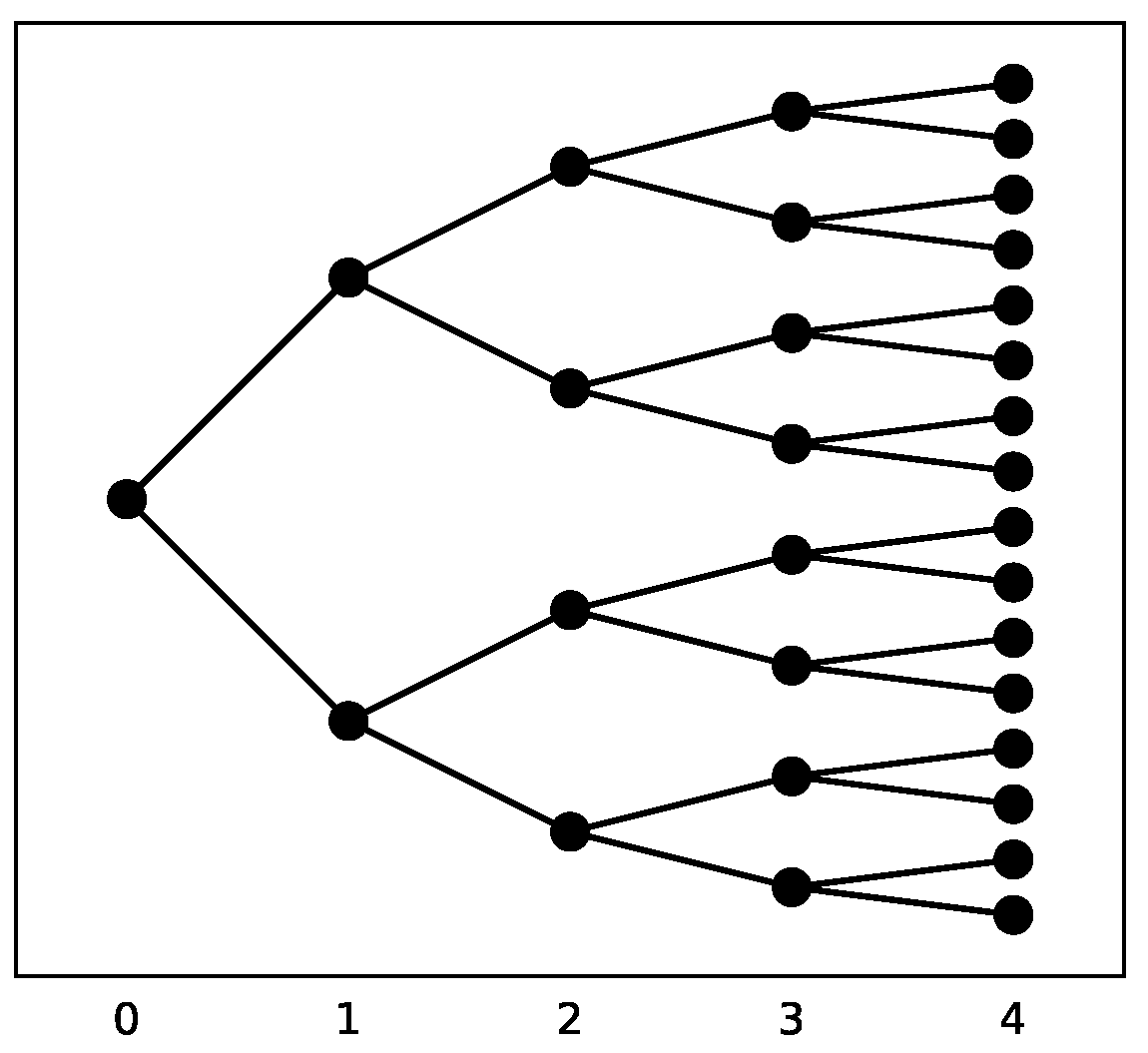
Figure 2. Exponential growth

$e^t$

. (a) Linear plot. (b) Semi-log plot.

Figure 2. Exponential growth

$e^t$

. (a) Linear plot. (b) Semi-log plot.

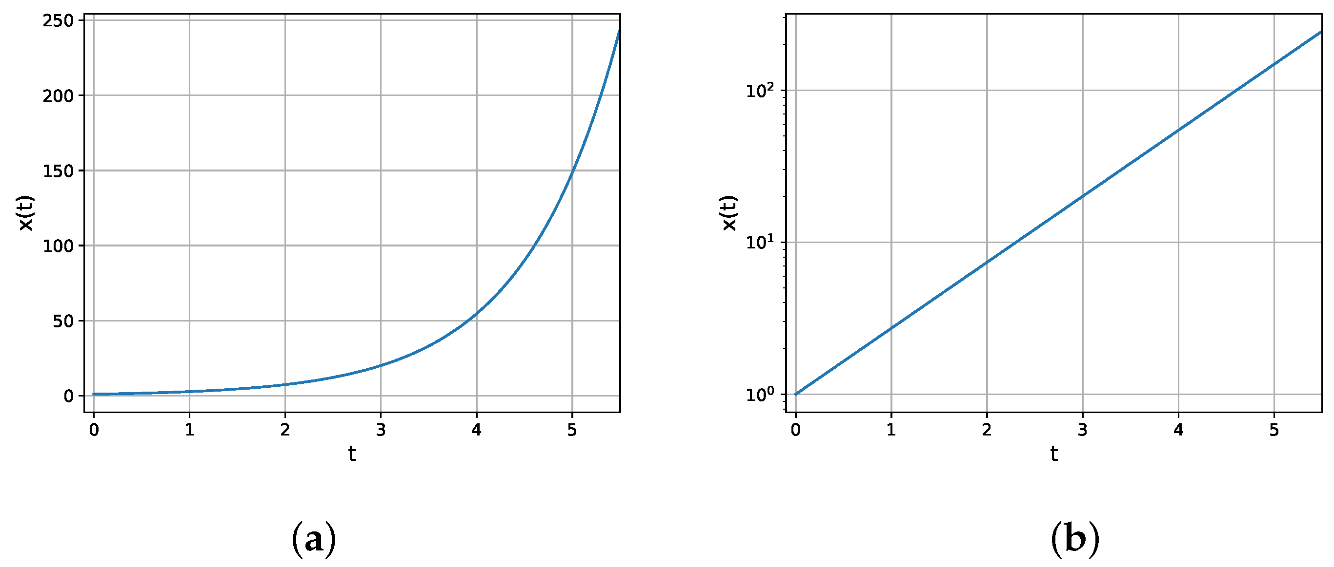
Figure 3. The numerical solution of the SIR model using the Runge–Kutta method;

$N=10,000,N_1=9900,N_2=10,N_3=0$

. (a) Plot of the temporal variation of the susceptible (S), the infected (I), and the recovered (R) for

$\beta =0.5$

and

$\gamma =0.2$

. In addition, the number of the newly infected individuals is shown by the red dotted curve. The time-dependent

$R_0\left(t\right)$

is also shown in the black dashed curve. (b) The comparison of S, I, R for

$\beta$

=0.5, 0.45, 0.4, 0.35, and 0.3;

$\gamma$

is fixed as 0.2.

Figure 3. The numerical solution of the SIR model using the Runge–Kutta method;

$N=10,000,N_1=9900,N_2=10,N_3=0$

. (a) Plot of the temporal variation of the susceptible (S), the infected (I), and the recovered (R) for

$\beta =0.5$

and

$\gamma =0.2$

. In addition, the number of the newly infected individuals is shown by the red dotted curve. The time-dependent

$R_0\left(t\right)$

is also shown in the black dashed curve. (b) The comparison of S, I, R for

$\beta$

=0.5, 0.45, 0.4, 0.35, and 0.3;

$\gamma$

is fixed as 0.2.

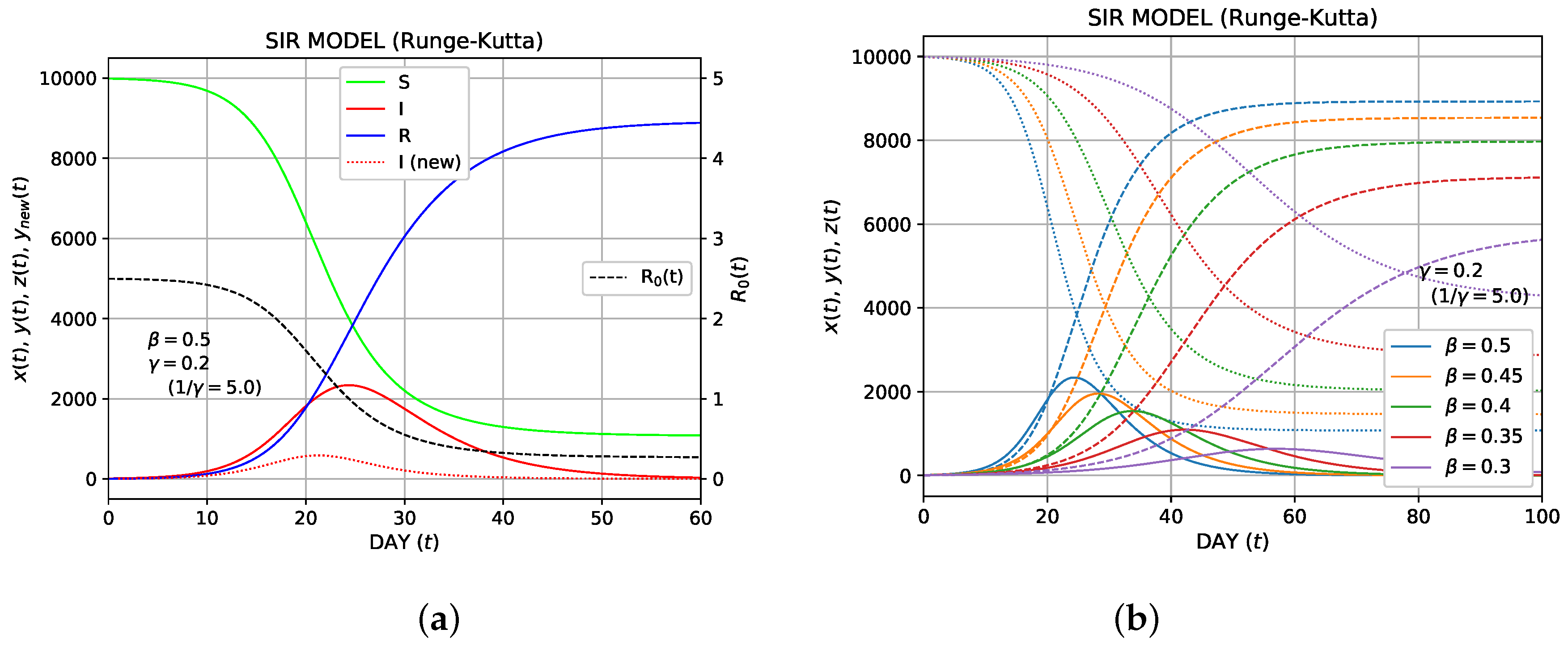
Figure 4. The semi-log plot of the cumulative number of the infected, (

$y\left(t\right)+z\left(t\right))$

.

Figure 4. The semi-log plot of the cumulative number of the infected, (

$y\left(t\right)+z\left(t\right))$

.

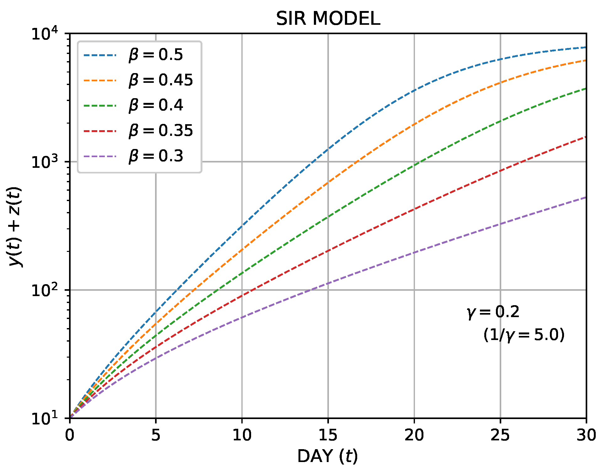
Figure 5. The analytical solution of the SIR model. The conditions are the same as in Figure 3a.

Figure 5. The analytical solution of the SIR model. The conditions are the same as in Figure 3a.

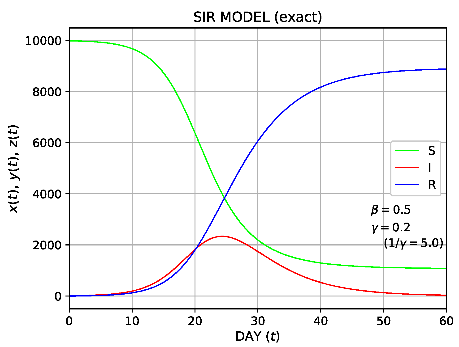
Figure 6. The solution of Equation (54).

Figure 6. The solution of Equation (54).

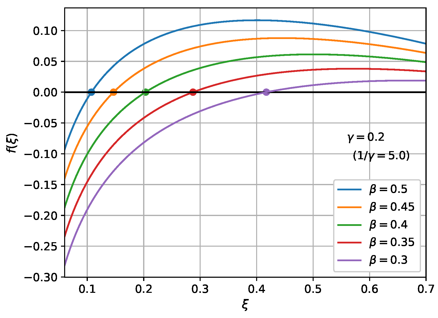
Figure 7. The solution of the SIR model with vital dynamics. The parameter

$\mu$

is varied as 0.0, 0.02, 0.04, 0.06, and 0.08, and the data of

$\mu =0.0$

are shown by thick dashed curves.

Figure 7. The solution of the SIR model with vital dynamics. The parameter

$\mu$

is varied as 0.0, 0.02, 0.04, 0.06, and 0.08, and the data of

$\mu =0.0$

are shown by thick dashed curves.

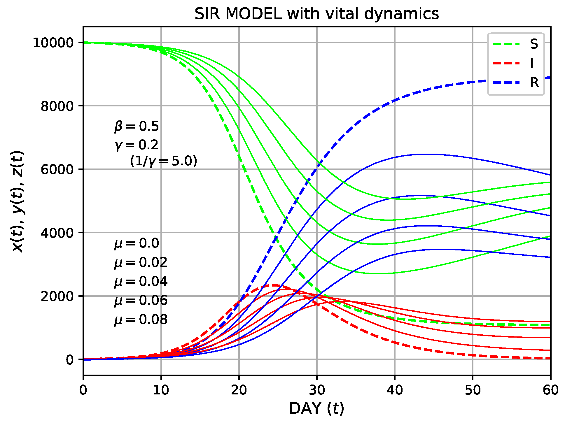
Table 1. The final number of the infected individuals: N = 10,000,

$N_1$

= 9900,

$N_2$

= 10,

$N_3$

= 0,

$\gamma$

is fixed as 0.2. The peak values of the infected individuals are also shown.

Table 1. The final number of the infected individuals: N = 10,000,

$N_1$

= 9900,

$N_2$

= 10,

$N_3$

= 0,

$\gamma$

is fixed as 0.2. The peak values of the infected individuals are also shown.

	The Final Number	The Infected ($\mathit{y}\left(\mathit{t}\right)$)		The Newly Infected (${\mathit{y}}_{\mathbf{new}}\left(\mathit{t}\right)$)
	of the Infected	Peak Day	Peak Number	Peak Day	Peak Number
$\beta$ = 0.50 ($R_0$ = 2.5)	8916	24.4	2339	21.2	587
$\beta$ = 0.45 ($R_0$ = 2.25)	8524	28.3	1956	24.9	468
$\beta$ = 0.40 ($R_0$ = 2.0)	7958	33.8	1539	30.2	351
$\beta$ = 0.35 ($R_0$ = 1.75)	7117	42.2	1094	38.4	238
$\beta$ = 0.30 ($R_0$ = 1.5)	5818	57.0	637	52.8	133

© 2020 by the authors. Licensee MDPI, Basel, Switzerland. This article is an open access article distributed under the terms and conditions of the Creative Commons Attribution (CC BY) license (http://creativecommons.org/licenses/by/4.0/).

We use cookies on our website to ensure you get the best experience.
Read more about our cookies here.

We have just recently launched a new version of our website.
Help us to further improve by taking part in this short 5 minute survey here. here.

Mathematical Models In Population Biology And Epidemiology Solutions Manual Pdf

Source: https://www.mdpi.com/2227-7390/8/7/1174/htm

Posted by: bowlesarned1981.blogspot.com

Share this post